Sea Surface leveling (SSL)

ForWind Oldenburg Version 1.0

Contributing author: Andreas Rott

To understand the calculations and methods presented in this notebook it is highly recommended to read the corresponding publication: Rott, A., Schneemann, J., Theuer, F., Trujillo Quintero, J. J., and Kühn, M.: Alignment of scanning lidars in offshore wind farms, Wind Energ. Sci. Discuss. [preprint], https://doi.org/10.5194/wes-2021-62, in review, 2021.

Executed with Python 3.8.12

TOC

0. Import

1. Load Data

   1. Load Lidar Data

   2. Load SCADA Data

2. SSL

   1. Estimate intersection of the lidar beam with the sea surface

      1. Example

   2. Model intersection of the lidar beam with the sea surface

      1. Example

   3. Fit model to estimate

      1. Example

3. Apply SSL to Lidar Data

   1. Compare heights with measurements from BSH

4. Platform Tilt Model

   1. Apply Thrust model to SSL results

   2. Calculate tilt angle from thrust model

   3. Calculate tilt angle from SSL measurements

   4. Compare tilt angles from thrust model and from SSL

   5. Calculate modelled roll and pitch from thrust model

5. Evaluate Results

6. Extra: Alternative Methode based on vectorial calculation

0. Imports

# Imports
import numpy as np
import pandas as pd
from scipy.optimize import minimize
from scipy.optimize import Bounds
import matplotlib.pyplot as plt
import sympy as sp
from tqdm import tqdm

1. Load Data

# file path to the lidar and the scada data
lidar_file_path = 'https://zenodo.org/record/5654866/files/SSL_scans_GTI.zip'
scada_file_path = 'https://zenodo.org/record/5654866/files/SCADA_rand_norm.csv'
ssh_gt1_file_path = 'https://zenodo.org/record/5654866/files/SSH_GTI.txt'
df_results_file_path = 'https://zenodo.org/record/5654866/files/df_results_SSL.zip'

1.1 Load Lidar Data

# df_lidar = pd.read_csv(lidar_file_path,index_col='datetime',parse_dates=['datetime'])
df_lidar = pd.read_pickle(lidar_file_path)

print('Number of scans: {}'.format(df_lidar.scan_nr.max()))
print('Start Date: {}'.format(df_lidar.index.min()))
print('End Date: {}'.format(df_lidar.index.max()))

Number of scans: 2493
Start Date: 2019-04-11 08:31:33
End Date: 2019-05-17 11:18:05

1.2 Load SCADA Data

Scada Data is only needed for the Platform Tilt Model (Section 4.1). For the SSL only the lidar data is required

df_scada = pd.read_csv(scada_file_path, index_col = 'Timestamp', parse_dates=['Timestamp'])
print('Start Date: {}'.format(df_scada.index.min()))
print('End Date: {}'.format(df_scada.index.max()))

Start Date: 2019-04-10 00:00:00
End Date: 2019-05-17 23:59:59

2. SSL

2.1 Distance to water Function

This function estimates the distance from the lidar device to the intersection of the beam with the sea surface for each individual azimut angle.
The inputs are the lidar data [data], a threshold for a minimal cnr value [min_cnr], which filters out scans, that do not reach this cnr value for any range gate and an optional variable [show_plot], which can be set to display the results of the estimated distance.
Further in this function the upper bounds (ub) and lower bounds (lb) for the parameters of the fit function need be specified. These bounds ensure that the automatic estimation is within reasonable limits. The bounds depend on the setup of the sea surface leveling scan and on the lidar device.
The [high_cnr_ub] and [high_cnr_lb] represent the limits for the average cnr values before the beam hits the sea surface.
The [low_cnr_ub] and [low_cnr_lb] represent the limits for the average cnr values for ranges bigger than the distance to the sea surface, which is practically the background noise of the device.
The [distance_ub] and [distance_lb] give the upper and lower bound for the distance to the intersection of the beam with the sea surface.
The growth rate of the inverse logistic funciton is limited by the parameters [growth_ub] and [growth_lb]. In our experience a growth rate between 0 and 1 is reasonable for our setup.

def distance_to_water(data,min_cnr,show_plot=0,high_cnr_ub=0,high_cnr_lb=-25,low_cnr_ub=-15,low_cnr_lb=-30,distance_ub=550,distance_lb=400,growth_ub=1,growth_lb=0):
    azis = data.azi.unique()
    distances = np.array([])
    for azi in azis:
        data_act = data[data.azi==azi]
        if data_act.cnr.max()<min_cnr:
            distance = np.nan
        else:
            fit_function = lambda up,down,mid,growth: (up-down)/(1+np.exp((data_act.range-mid)*growth))+down
            cost_function = lambda param: np.sum((data_act.cnr-fit_function(param[0],param[1],param[2],param[3]))**2)
            bounds = Bounds([high_cnr_lb,low_cnr_lb,distance_lb,growth_lb],[high_cnr_ub,low_cnr_ub,distance_ub,growth_ub])
            
            # initial guess for parameters of the inverse sigmoid function
            high_cnr = data_act.cnr.max()
            low_cnr = data_act.cnr.min()
            middle_cnr = (high_cnr+low_cnr)/2
            min_distance = data_act.range[data_act.cnr > middle_cnr].min()
            middle_range = data_act.range[(data_act.range > min_distance) & (data_act.cnr<=middle_cnr)].min()

            res = minimize(cost_function,[high_cnr,low_cnr,middle_range,0.1],bounds=bounds)
#             print(res)
            if res.x[0]<min_cnr-3:
                distance=np.nan
            else:
                distance = res.x[2]
            if show_plot:
                ax = data_act.plot('range','cnr',grid=True,legend=False,figsize=(12/2.54,9/2.54),linewidth=2,style='.',color='r')
                ax.set_ylabel('CNR')
                fig = ax.get_figure()
                fig.tight_layout()
                ax.set_xlabel('$r_\mathrm{lidar}$ [m]')
                ax.set_ylabel('CNR [dB]')
                ax.plot(data_act.range,fit_function(res.x[0],res.x[1],res.x[2],res.x[3]),linewidth=2,color='k')
                ax.vlines(res.x[2],data_act['cnr'].min()-1,data_act['cnr'].max()+1)
                ax.autoscale(enable=True, axis='both', tight=True)
                plt.show()
                print(f"high cnr: {res.x[0]} dB, low_cnr: {res.x[1]} dB, growth_rate: {res.x[3]}")
                print(f"Azimut Angle: {azi}° and estimated distance: {distance} m")
        distances = np.append(distances,distance)
    return azis[~np.isnan(distances)],distances[~np.isnan(distances)]

2.1.1 Example for distance to water estimation

df_lidar_example = df_lidar[df_lidar.scan_nr == 1105].sort_values(['azi','range']).copy()

A,D = distance_to_water(df_lidar_example[df_lidar_example.azi == df_lidar_example.azi.unique()[80]],-18,show_plot=1) # use this to show the estimation for just one azimut angle
# A,D = distance_to_water(df_lidar_example,-18,show_plot=1)  # use this to show the estimation for every azimut angle

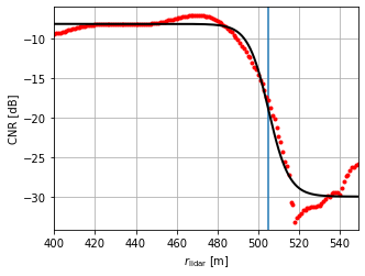
high cnr: -8.133507278433605 dB, low_cnr: -29.980503797298205 dB, growth_rate: 0.19891362652575575
Azimut Angle: 234.662° and estimated distance: 505.087954191345 m

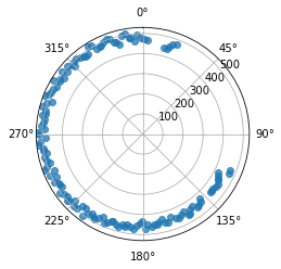
A,D = distance_to_water(df_lidar_example,-18)
fig,ax= plt.subplots(1,1,subplot_kw=dict(polar=True),figsize=(12/2.54,9/2.53))
ax.scatter(A/180*np.pi,D, cmap='hsv', alpha=0.75)
ax.set_theta_zero_location("N")
ax.set_theta_direction(-1)
ax.set_rlabel_position(50)
fig.tight_layout()

2.2 Model intersection of lidar with sea surface

in the next cells the mathematical derivation of the formula for the intersection of the ppi scan with the water surface is shown

# Rotational matrices
M_x = lambda x: sp.Matrix([[1,0,0],[0, sp.cos(x),sp.sin(x)],[0,-sp.sin(x),sp.cos(x)]])
M_y = lambda x: sp.Matrix([[sp.cos(x),0,-sp.sin(x)],[0,1,0],[sp.sin(x),0,sp.cos(x)]])
M_z = lambda x: sp.Matrix([ [sp.cos(x) ,sp.sin(x) ,0 ],[-sp.sin(x) ,sp.cos(x) ,0 ],[ 0, 0, 1]])
alpha = sp.Symbol('alpha')
display(M_x(alpha))
display(M_y(alpha))
display(M_z(alpha))

\[\begin{split}\displaystyle \left[\begin{matrix}1 & 0 & 0\\0 & \cos{\left(\alpha \right)} & \sin{\left(\alpha \right)}\\0 & - \sin{\left(\alpha \right)} & \cos{\left(\alpha \right)}\end{matrix}\right]\end{split}\]

\[\begin{split}\displaystyle \left[\begin{matrix}\cos{\left(\alpha \right)} & 0 & - \sin{\left(\alpha \right)}\\0 & 1 & 0\\\sin{\left(\alpha \right)} & 0 & \cos{\left(\alpha \right)}\end{matrix}\right]\end{split}\]

\[\begin{split}\displaystyle \left[\begin{matrix}\cos{\left(\alpha \right)} & \sin{\left(\alpha \right)} & 0\\- \sin{\left(\alpha \right)} & \cos{\left(\alpha \right)} & 0\\0 & 0 & 1\end{matrix}\right]\end{split}\]

def create_fit_function():
    pitch_sym, roll_sym, height_sym, ele_sym, yaw_sym, range_sym, shift_x, shift_y = sp.symbols('phi rho h varepsilon gamma r s_x s_y')
    M_x = lambda x: sp.Matrix([[1,0,0],[0, sp.cos(x),sp.sin(x)],[0,-sp.sin(x),sp.cos(x)]])
    M_y = lambda x: sp.Matrix([[sp.cos(x),0,-sp.sin(x)],[0,1,0],[sp.sin(x),0,sp.cos(x)]])
    M_z = lambda x: sp.Matrix([ [sp.cos(x) ,sp.sin(x) ,0 ],[-sp.sin(x) ,sp.cos(x) ,0 ],[ 0, 0, 1]])

    laser_beam = lambda x: sp.Matrix([[0],[x],[0]])
    Pitch = M_x(pitch_sym)
    Roll = M_y(roll_sym)
    Yaw = M_z(yaw_sym)
    Ele = M_x(-ele_sym)
    Laser_beam = laser_beam(range_sym)
    Shift = sp.Matrix([[shift_x],[shift_y],[0]])
    Height = sp.Matrix([[0],[0],[height_sym]])
    lidar = Height + Pitch * Roll* Yaw * (Ele * Laser_beam + Shift )
    
    display(0)
    print('=')
    display(lidar[2])
    result = sp.solve(lidar[2],range_sym)
    print('')
    display(range_sym)
    print('=')
    display(result[0])
    return
create_fit_function()

0

=

\[\displaystyle h + r \sin{\left(\varepsilon \right)} \cos{\left(\phi \right)} \cos{\left(\rho \right)} + s_{x} \left(\sin{\left(\gamma \right)} \sin{\left(\phi \right)} + \sin{\left(\rho \right)} \cos{\left(\gamma \right)} \cos{\left(\phi \right)}\right) + \left(r \cos{\left(\varepsilon \right)} + s_{y}\right) \left(\sin{\left(\gamma \right)} \sin{\left(\rho \right)} \cos{\left(\phi \right)} - \sin{\left(\phi \right)} \cos{\left(\gamma \right)}\right)\]

\[\displaystyle r\]

=

\[\displaystyle \frac{h + s_{x} \sin{\left(\gamma \right)} \sin{\left(\phi \right)} + s_{x} \sin{\left(\rho \right)} \cos{\left(\gamma \right)} \cos{\left(\phi \right)} + s_{y} \sin{\left(\gamma \right)} \sin{\left(\rho \right)} \cos{\left(\phi \right)} - s_{y} \sin{\left(\phi \right)} \cos{\left(\gamma \right)}}{- \sin{\left(\gamma \right)} \sin{\left(\rho \right)} \cos{\left(\phi \right)} \cos{\left(\varepsilon \right)} + \sin{\left(\phi \right)} \cos{\left(\gamma \right)} \cos{\left(\varepsilon \right)} - \sin{\left(\varepsilon \right)} \cos{\left(\phi \right)} \cos{\left(\rho \right)}}\]

def fit_function(pitch, roll, height, ele, yaw, s_x = -0.15, s_y = 0.15):
    return (
        height +
        s_x*np.sin(yaw/180*np.pi)*np.sin(pitch/180*np.pi)+
        s_x*np.sin(roll/180*np.pi)*np.cos(yaw/180*np.pi)*np.cos(pitch/180*np.pi)+
        s_y*np.sin(yaw/180*np.pi)*np.sin(roll/180*np.pi)*np.cos(pitch/180*np.pi)-
        s_y*np.sin(pitch/180*np.pi)*np.cos(yaw/180*np.pi)
    )/(
        np.cos(ele/180*np.pi)*
        (
            np.cos(yaw/180*np.pi)*np.sin(pitch/180*np.pi)-
            np.cos(pitch/180*np.pi)*np.sin(roll/180*np.pi)*np.sin(yaw/180*np.pi)        
        )-
        np.cos(pitch/180*np.pi)*np.cos(roll/180*np.pi)*np.sin(ele/180*np.pi)
    )

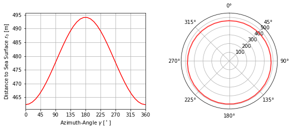
2.2.1 Example for modelled intersection

Here is an example sea surface intersection with a pitch angle of 0.1 Degree at a height of 25 m and an elevation of -3 Degree. Such a small misalignment leads to quite big differences in the distances, opposed to a perfectly alignd device which yields a perfect circle.

yaw=np.linspace(start=0,stop=359,num=36)
D = fit_function(pitch=0.1,roll=0,height=25,ele=-3,yaw=yaw)

fig = plt.figure(figsize =(24/2.54,9/2.54))
# left figure
ax2 = plt.subplot(121)
ax2.plot(yaw,D,'r',label=r'$r_0$')
ax2.grid(True)
ax2.set_xlabel('Azimuth-Angle $\gamma\ [^\circ]$')
ax2.set_ylabel('Distance to Sea Surface $r_0\ [\mathrm{m}]$')
ax2.set_xticks(np.arange(0,361,step=45))
ax2.set_xlim(0,360)
# right figure
ax1 = plt.subplot(122, projection='polar')
ax1.grid(True)
ax1.plot(yaw/180*np.pi,D,'r', alpha=0.75,linewidth=2,label=r'$r_0$' )
ax1.set_theta_zero_location("N")
ax1.set_theta_direction(-1)
ax1.set_rlabel_position(45)
ax1.set_ylim(0,550)

(0.0, 550.0)

2.3 Fit Model to Estimate (SSL function)

Here we use an optimization to find the best parameters (pitch, roll and height) which reflect the measured distances best

• lorentz optimization for better outlier tolerance

def lidar_alignment(data,minimum_cnr,approx_height_above_nn):
    Azi,Distance = distance_to_water(data,minimum_cnr)
    start_time = data.index.min()
    if all(data.ele>-3.01) and all(data.ele<-2.99) and len(Azi)>20:
        ele = -3
    else:
        return np.nan, np.nan, np.nan, np.nan,np.nan, np.nan
    
    x0 = [0,0,approx_height_above_nn]
#     method = 'least-squares'
    method = 'lorentz'
    if method == 'lorentz':
        Cost = lambda x: np.sum(
            np.log(
                1+0.5*(
                    Distance - fit_function(pitch=x[0],roll=x[1],height=x[2],ele=ele,yaw=Azi)
                )**2
            )
        )
    elif method == 'least-squares':
        Cost = lambda x: np.sum(
            (
                Distance - fit_function(pitch=x[0],roll=x[1],height=x[2],ele=ele,yaw=Azi)
            )**2
        )   
    res = minimize(Cost, x0, method='nelder-mead',options={'xatol': 1e-8, 'disp': False})
    p,r,h = res.x
    return p,r,h,Azi,Distance, start_time
        

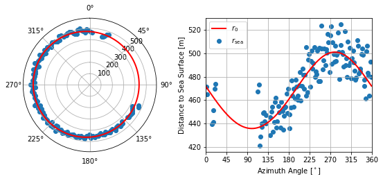
2.3.1 Example for SSL on exemplary Lidar Scan

Here we apply the optimization to the example data, together with the distance_to_water to compare the model results to the measured water distances.

p,r,h,Azi,Distance, start_time=lidar_alignment(df_lidar_example,-18,25)
Azi,Distance = distance_to_water(df_lidar_example,-18)

fig = plt.figure(figsize=(24/2.54,9/2.54))
ax1 = plt.subplot(121,projection='polar')
ax1.scatter(Azi/180*np.pi,Distance)
ax1.set_theta_zero_location("N")
ax1.set_theta_direction(-1)
ax1.set_rlabel_position(45)
ax1.plot(np.arange(0,360)/180*np.pi,fit_function(p,r,h,-3,np.arange(0,360)),'r',linewidth=2)
ax1.grid(True)
ax1.set_ylim(0,590)

ax2 = plt.subplot(122)
ax2.scatter(Azi,Distance,label=r'$r_\mathrm{sea}$')
ax2.plot(np.arange(0,360),fit_function(p,r,h,-3,np.arange(0,360)),'r',linewidth=2,label=r'$r_0$')
ax2.grid(True)
ax2.set_xlabel('Azimuth Angle $[^\circ]$')
ax2.set_xticks(np.arange(0,361,step=45))
ax2.set_ylabel('Distance to Sea Surface [m]')
ax2.set_xlim(0,360)
ax2.legend()
print(p,r,h)

-0.034234773554786144 -0.20599689693051043 24.396504475562985

3. Apply SSL to Lidar Data

Here the lidar alignment is applied on the whole data set. This means for each SSL scan the Fit-model is applied to estimate the leveling, for this the distances for every azimut angle in every scan needs to be estimated. Depending on the number of scans this can take several hours. For this reason, we have saved the results in a df_results_SSL.zip file to faster progress through the code.
The variable [do_the_calculation] lets you recalculate the results and overwrites the df_results_SSL.zip file with the new results.

# The calculation of a single sea surface scan takes about 40 s. 
# To calculate the entire example data set the calculation takes several hours. 
# Therefore we pre calculated the results and stored them in a zip file.
do_the_calculation = False  
if do_the_calculation:
    P = np.array([])
    R = np.array([])
    H = np.array([])
    T = np.array([])
    df_results_SSL = pd.DataFrame()
    for scan_nr in tqdm(df_lidar.scan_nr.unique()):
        idx = (df_lidar.scan_nr == scan_nr)
        p,r,h,Azi,Distance, t=lidar_alignment(df_lidar[idx],-18,25)
        if any([np.isnan(p),np.isnan(r),np.isnan(h)]):
            continue
        else:
            P = np.append(P,p)
            R = np.append(R,r)
            H = np.append(H,h)
            T = np.append(T,t)
    df_results_SSL = pd.DataFrame({'pitch':P,'roll':R,'height':H},index=T)
    # df_results_SSL.to_pickle('df_results_SSL.zip')
else:
    df_results_SSL = pd.read_pickle(df_results_file_path)
len(df_results_SSL)

1930

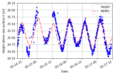
3.1 Compare heights with measurements from BSH

ssh = pd.read_csv(ssh_gt1_file_path,sep='\s+', header=None,names=['date','ssh'])
ssh.set_index(pd.to_datetime(ssh.date,format='%Y%m%d%H%M'),inplace=True)
ssh.drop(['date'],axis=1,inplace=True)
df_results_SSL = df_results_SSL.join(ssh,how='outer')
cost = lambda x: np.sum((df_results_SSL.height.resample('1h').mean() + df_results_SSL.ssh.resample('1h').mean()-x)**2)
opt_height_diff = minimize(cost,0)
opt_h = opt_height_diff.x
print('height above sea surface: {:.2f} m'.format(opt_h[0]))
df_results_SSL.ssh[pd.notna(df_results_SSL.ssh)] = opt_h - df_results_SSL.ssh[pd.notna(df_results_SSL.ssh)]

height above sea surface: 24.83 m

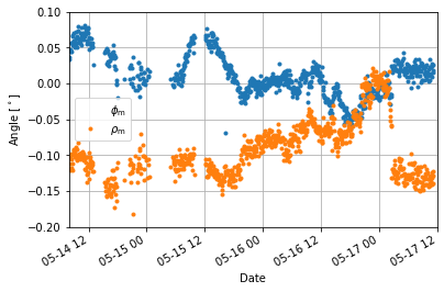
ax1 = df_results_SSL['pitch'].plot(style='.',label=r'$\phi_\mathrm{m}$',legend=True, grid=True)
df_results_SSL['roll'].plot(style='.',label=r'$\rho_\mathrm{m}$',legend=True, grid=True)
start_time = pd.Timestamp('2019-05-14 08:00')
end_time = pd.Timestamp('2019-05-17 12:00')
ax1.set_xlim(start_time, end_time)
ax1.set_ylim(-0.2, 0.1)
ax1.set_ylabel('Angle $[^\circ]$')
ax1.set_xlabel('Date')
plt.show()

ax2 = df_results_SSL['height'].plot(style='.',c='b', legend=True,grid=True)
df_results_SSL['ssh'][pd.notna(df_results_SSL['ssh'])].plot(style='-.',c='r',legend=True,label='NEMO',zorder=2,grid=True)
ax2.set_xlim(start_time, end_time)
ax2.set_ylim(24.25,26.25)
ax2.set_ylabel('Height above sea surface $h$ [m]')
ax2.set_xlabel('Date')
plt.show()

4. Platform Tilt Model (PTM)

The PTM attempts to relate the leveling of the transition piece to the thrust of the turbine. We have the measured instantaneous leveling given by the two angles $\phi_\mathrm{m}$ (measured pitch angle) and $\rho_\mathrm{m}$ (measured roll angle). To construct the PTM we need to determine the follwoing three variables: $\phi_\mathrm{r}$ (pitch angle at rest, i. e. without thrust), $\rho_\mathrm{r}$ (roll angle at rest) and the variable $\tau$, which is a linear scaling factor for the thrust of the wind turbine.

pitch_m, roll_m, pitch_r, roll_r, tilt, yaw = sp.symbols('phi_m rho_m phi_r rho_r tau gamma')

Pitch_m = M_x(pitch_m)
Roll_m = M_y(roll_m)
Pitch_r = M_x(pitch_r)
Roll_r = M_y(roll_r)
Tilt = M_z(yaw)*M_x(-tilt)*M_z(-yaw)

Left = Pitch_m*Roll_m*sp.Matrix([[0],[0],[1]])
Right = Tilt*Pitch_r*-Roll_r*sp.Matrix([[0],[0],[1]])

display(Left-Right)

\[\begin{split}\displaystyle \left[\begin{matrix}\left(\left(\sin{\left(\gamma \right)} \cos{\left(\gamma \right)} \cos{\left(\tau \right)} - \sin{\left(\gamma \right)} \cos{\left(\gamma \right)}\right) \sin{\left(\phi_{r} \right)} - \sin{\left(\gamma \right)} \sin{\left(\tau \right)} \cos{\left(\phi_{r} \right)}\right) \cos{\left(\rho_{r} \right)} - \left(\sin^{2}{\left(\gamma \right)} \cos{\left(\tau \right)} + \cos^{2}{\left(\gamma \right)}\right) \sin{\left(\rho_{r} \right)} - \sin{\left(\rho_{m} \right)}\\\left(\left(\sin^{2}{\left(\gamma \right)} + \cos^{2}{\left(\gamma \right)} \cos{\left(\tau \right)}\right) \sin{\left(\phi_{r} \right)} - \sin{\left(\tau \right)} \cos{\left(\gamma \right)} \cos{\left(\phi_{r} \right)}\right) \cos{\left(\rho_{r} \right)} - \left(\sin{\left(\gamma \right)} \cos{\left(\gamma \right)} \cos{\left(\tau \right)} - \sin{\left(\gamma \right)} \cos{\left(\gamma \right)}\right) \sin{\left(\rho_{r} \right)} + \sin{\left(\phi_{m} \right)} \cos{\left(\rho_{m} \right)}\\\left(\sin{\left(\phi_{r} \right)} \sin{\left(\tau \right)} \cos{\left(\gamma \right)} + \cos{\left(\phi_{r} \right)} \cos{\left(\tau \right)}\right) \cos{\left(\rho_{r} \right)} - \sin{\left(\gamma \right)} \sin{\left(\rho_{r} \right)} \sin{\left(\tau \right)} + \cos{\left(\phi_{m} \right)} \cos{\left(\rho_{m} \right)}\end{matrix}\right]\end{split}\]

M_x(pitch_m)*M_y(roll_m)*sp.Matrix([[0],[0],[1]])

\[\begin{split}\displaystyle \left[\begin{matrix}- \sin{\left(\rho_{m} \right)}\\\sin{\left(\phi_{m} \right)} \cos{\left(\rho_{m} \right)}\\\cos{\left(\phi_{m} \right)} \cos{\left(\rho_{m} \right)}\end{matrix}\right]\end{split}\]

The tilt was converted into a lot vector. From this, pitch and roll can be calculated again. It applies: $$ \begin{pmatrix} x\ y\ z\ \end{pmatrix}= M_x(\phi)\cdot M_y(\rho) \cdot \begin{pmatrix} 0 \ 0 \ 1 \end{pmatrix}= \begin{pmatrix} -\sin(\rho)\ \cos(\rho)\sin(\phi)\ \cos(\rho)\cos(\phi) \end{pmatrix} $$

With this you can invert the equation: $\rho = \arcsin(-x)$ und $\phi = \arcsin\left(\frac{y}{\cos(\rho)}\right)$

4.1 Apply PTM to SSL results

Estimate resting pitch and roll and lin scaling factor

df = df_scada.join(df_results_SSL)
df = df.resample('5min').mean()
df = df[~df['pitch'].isna()]
df.reset_index(inplace=True)
df.loc[:,'PitchB1'] = df.loc[:,'PitchB1'].ffill()

M_x = lambda x: np.array([[1,0,0],[0, np.cos(x/180*np.pi),np.sin(x/180*np.pi)],[0,-np.sin(x/180*np.pi),np.cos(x/180*np.pi)]],dtype="object")
M_y = lambda x: np.array([[np.cos(x/180*np.pi),0,-np.sin(x/180*np.pi)],[0,1,0],[np.sin(x/180*np.pi),0,np.cos(x/180*np.pi)]],dtype="object")
M_z = lambda x: np.array([ [np.cos(x/180*np.pi) ,np.sin(x/180*np.pi) ,0 ],[-np.sin(x/180*np.pi) ,np.cos(x/180*np.pi) ,0 ],[ 0, 0, 1]],dtype="object")

pitch_m = np.array(df['pitch'])
roll_m = np.array(df['roll'])
u = np.array(df['WSpd'])
p = np.array(df['P'])
yaw = np.array(df['NacPos'])

thrust = lambda power, wspd: np.where(power/wspd>0,power/wspd,0)

x0 = [0,0,0] 

cost = lambda x: np.linalg.norm(
    np.linalg.norm(
        M_z(yaw)@M_x(-x[0]*thrust(p,u))@M_z(-yaw)@M_x(x[1])@M_y(x[2])-M_x(pitch_m)@M_y(roll_m)
    ).squeeze()
)

result_opt = minimize(cost,np.array(x0),method='Nelder-Mead')

result_opt

 final_simplex: (array([[ 1.85417296,  0.02580108, -0.11284461],
       [ 1.85423953,  0.02580327, -0.11284274],
       [ 1.85418547,  0.02579989, -0.11284318],
       [ 1.85410942,  0.02580087, -0.11284318]]), array([0.02397691, 0.02397691, 0.02397691, 0.02397691]))
           fun: 0.02397691355116423
       message: 'Optimization terminated successfully.'
          nfev: 283
           nit: 158
        status: 0
       success: True
             x: array([ 1.85417296,  0.02580108, -0.11284461])

a, pitch_r, roll_r  = result_opt.x

4.2 Calculate tilt angle from thrust model

df['tilt']=a*thrust(p,u)

4.3 Calculate tilt angle from SSL measurements

pitch_measured = np.array(df['pitch'])
roll_measured = np.array(df['roll'])
yaw_turbine = np.array(df['NacPos'])
pitch_rest = pitch_r
roll_rest = roll_r
x0 = 0
res_array=[]
for p,r,y in zip(pitch_measured, roll_measured,yaw_turbine):
    cost = lambda x: np.linalg.norm(
    np.linalg.norm(
        M_x(p)@M_y(r)-M_z(y)@M_x(-x)@M_z(-y)@M_x(pitch_rest)@M_y(roll_rest)
    ).squeeze()
    )
    result_opt_test = minimize(cost,0.14,method='Nelder-Mead')
    res_array.append(result_opt_test.x)
res_array = np.stack(res_array)
df['tilt_measured']=res_array

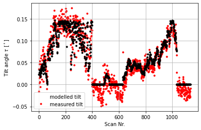
4.4 Compare tilt angles from thrust model and from SSL

ax = df['tilt'].plot(grid=True,c='k', style='.',label='modelled tilt',legend=True,zorder=2)
ax=df['tilt_measured'].plot(c='r',style='.',grid=True,label='measured tilt',legend=True, zorder=1)
ax.set_xlabel('Scan Nr.')
ax.set_ylabel(r'Tilt angle $\tau\ [^\circ]$')
plt.show()

from scipy.odr import *
from scipy.stats import linregress
def linear_func(p,x):
    m,c=p
    return m*x+c
linear_model = Model(linear_func)
data = RealData(np.array(df['P']/df['WSpd']),np.array(df['tilt_measured']))
odr = ODR(data,linear_model, beta0=[0.,1.])
out = odr.run()
out.pprint()

slope, intercept, r, p, se = linregress(np.array(df['P']/df['WSpd']),np.array(df['tilt_measured']))
print(slope,intercept)

Beta: [ 2.11165357 -0.01000501]
Beta Std Error: [0.0201143  0.00081163]
Beta Covariance: [[ 6.89200182 -0.21035195]
 [-0.21035195  0.01122149]]
Residual Variance: 5.870354116525627e-05
Inverse Condition #: 0.0026382848141896175
Reason(s) for Halting:
  Sum of squares convergence
1.945446408892748 -0.004932115554505213

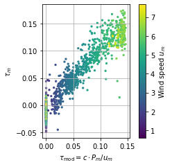
plt.figure(figsize=(12/2.54,9/2.54))
plt.scatter(df.sort_values(by=['WSpd'])['tilt'],df.sort_values(by=['WSpd'])['tilt_measured'],s=5,c=df.sort_values(by=['WSpd'])['WSpd'])
plt.xlabel(r'$\tau_{\mathrm{mod}} =c\cdot P_m / u_m$')
plt.ylabel(r'$\tau_m$')
plt.colorbar(label='Wind speed $u_m$')
plt.grid(True)
ax = plt.gca()
ax.set_aspect('equal')

4.5 Calculate modelled roll and pitch from thrust model

yaw = np.array(df['NacPos'])
tilt = np.array(df['tilt'])
X = M_z(yaw)@M_x(-tilt)@M_z(-yaw)@M_x(pitch_r)@M_y(roll_r)@np.matrix([[0],[0],[1]])

x = X[0,0].squeeze()
y = X[1,0].squeeze()
z = X[2,0].squeeze()

roll_mod = np.arcsin(-x)
pitch_mod = np.arcsin(y/np.cos(roll_mod))

df['roll_mod']=roll_mod/np.pi*180
df['pitch_mod']=pitch_mod/np.pi*180

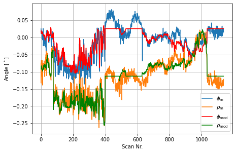
ax = df['pitch'].plot(grid=True, label=r'$\phi_\mathrm{m}$', legend=True,figsize=(18/2.54,12/2.54))
df['roll'].plot(grid=True, label=r'$\rho_\mathrm{m}$', legend=True)
(df['pitch_mod']).plot(grid=True,c='r', label='$\phi_\mathrm{mod}$', legend=True)
(df['roll_mod']).plot(grid=True,c='g', label=r'$\rho_\mathrm{mod}$', legend=True)
ax.set_xlabel('Scan Nr.')
ax.set_ylabel('Angle $[^\circ]$')
plt.show()

5. Evaluate Results

In this section we calculate the error statistics for the PTM

def rmse(input):
    return ((input**2).mean())**0.5

print('ROLL')
temp = df['roll']-df['roll_mod']
print(temp.describe())
print('rmse: ' +  str(rmse(df['roll']-df['roll_mod'])))
print('PITCH')
temp = df['pitch']-df['pitch_mod']
print(temp.describe())
print('rmse' + str(rmse(df['pitch']-df['pitch_mod'])))

ROLL
count    1137.000000
mean        0.000001
std         0.019279
min        -0.080147
25%        -0.012605
50%         0.000470
75%         0.012102
max         0.124606
dtype: float64
rmse: 0.019270046474657836
PITCH
count    1.137000e+03
mean     7.366210e-07
std      2.142424e-02
min     -9.375371e-02
25%     -1.182373e-02
50%     -6.137043e-04
75%      1.219341e-02
max      5.814154e-02
dtype: float64
rmse0.021414820443588844

6. Extra: Alternative Methode based on vectorial calculation

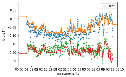
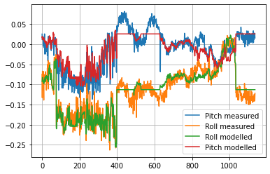
This section is just a bonus. Alternatively to the prior calculation it is possible to find a relation of the measured roll and pitch angles in the vector representation. For this we separate the thrust of the wind turbine into the vector components [Thrust_NS] along the $y$-axis and [Thrust_WE] along the $x$-axis. With this we try to find the linear relation between the pitch angle and the [Thrust_NS] and simulatiously between the roll-angle and [Thrust_WE].

df['Thrust_NS']=-np.cos(df['NacPos']/180*np.pi)*thrust(df['P'],df['WSpd'])
df['Thrust_WE']=-np.sin(df['NacPos']/180*np.pi)*thrust(df['P'],df['WSpd'])

cost = lambda x: np.sum(
    (np.array(df['pitch'])-np.array(x[1]+x[0]*df['Thrust_NS']))**2
)+np.sum(
    (np.array(df['roll'])-np.array(x[2]-x[0]*df['Thrust_WE']))**2
)

result_opt_vec = minimize(cost,[0,0,0],method='Nelder-Mead')
print(result_opt_vec)

 final_simplex: (array([[ 1.85417296,  0.02580108, -0.11284461],
       [ 1.85423953,  0.02580327, -0.11284274],
       [ 1.85418547,  0.02579989, -0.11284318],
       [ 1.85410942,  0.02580087, -0.11284318]]), array([0.94363005, 0.94363005, 0.94363005, 0.94363006]))
           fun: 0.9436300502206072
       message: 'Optimization terminated successfully.'
          nfev: 283
           nit: 158
        status: 0
       success: True
             x: array([ 1.85417296,  0.02580108, -0.11284461])

df['pitch_mod']=result_opt_vec.x[1]+result_opt_vec.x[0]*df['Thrust_NS']
df['roll_mod']=result_opt_vec.x[2]-result_opt_vec.x[0]*df['Thrust_WE']

ax=df['pitch'].plot(label='Pitch measured',legend=True,grid=True)
df['roll'].plot(label='Roll measured',legend=True,grid=True)
df['roll_mod'].plot(label='Roll modelled',legend=True,grid=True)
df['pitch_mod'].plot(label='Pitch modelled',legend=True,grid=True)
plt.show()

# Zoomed in plot
fig, ax  = plt.subplots()
start_time = pd.Timestamp('2019-05-02 08:00')
end_time = pd.Timestamp('2019-05-03 15:00')
ax.plot(df['index'],df['pitch'],'.')
ax.plot(df['index'],df['pitch_mod'])
ax.plot(df['index'],df['roll'],'.')
ax.plot(df['index'],df['roll_mod'])
ax.set_xlabel('measurements')
ax.set_ylabel('Angle $[^\circ]$')
ax.legend(['test'])
ax.set_xlim(start_time, end_time)
plt.show()