Hard Target Mapping (HTM) for elevation offset determination

To determine the elevation offset (and external misalignment = pitch/roll), we need to scan at least three distinct hard targets around the lidar with varying azimuth angles.

For each hard target, the polar coordinates are required from:

• lidar

• reference measurements (e.g., theodolite)

Positions of the hard targets in the lidar polar coordinate frame will be determined by the carrier to noise ratio (CNR) of the radial measurements. High CNR (>0dB) means a hard target is in the probe volume, whereas moderate CNR means that aerosols were detected in the probe volume.

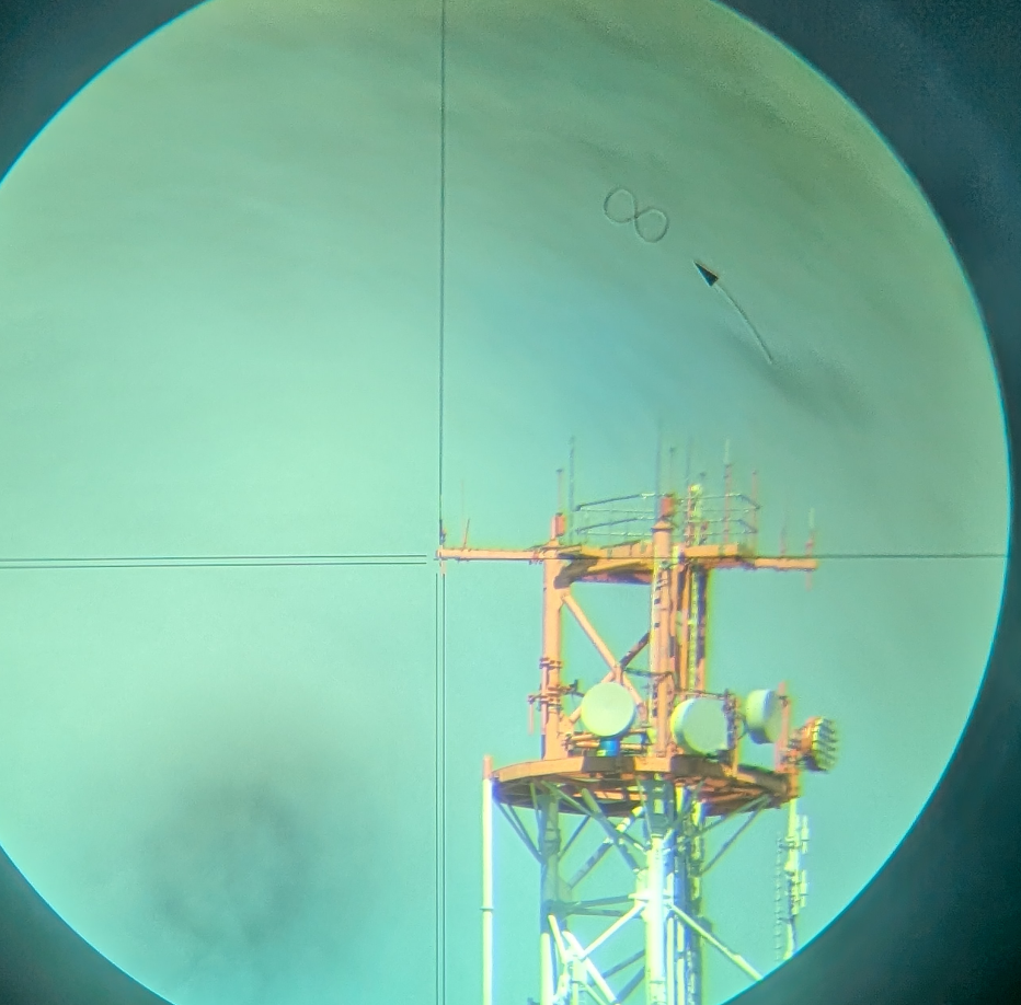
The actual Hard Target, measured with the Theodolite (foto taken through the theodolite lense):

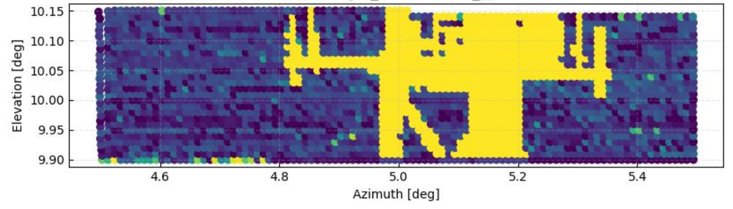
The same Hard Target, measured with the Lidar (yellow means high CNR >0dB, blue is low CNR of <-25dB>):

For a general overview about the hard target mapping (CNR mapper), see the initial description by Vasiljevic 2014.

Examplary demonstration

Let us imagine one example of a lidar installation, where multiple hard targets have been measured around the lidar.

First we import required packages.

import matplotlib.pyplot as plt
import numpy as np
import pandas as pd
import plotly.graph_objects as go
from lidalign.hard_target_elevation_mapping import HardTargetMappingElevation

Coordinate list

Imagine, we have performed multiple maps of hard targets and obtained reference coordinates using a theodolit:

data = {
    "Pt name": [
        "RADTOP", "ELECTROTOWER", "MAST L11",
        "MAST TOP1", "P1 HOUSE", "MAST L2"
    ],
    "Theo_Azimuth": ["123,6162", "159,9877", "247,1387", "247,1376", "210,3619", "247,1331"], # azimuth from theodolite
    "Theo_ElevationVert": ["89,2637", "89,6018", "87,0018", "87,0143", "90,1346", "87,5357"], # Elevation from vertical (vertical = 0°) from theodolit
    "Lidar_azim": ["123,96", "160,285", "247,43", "", "210,6", "247,43"], # Azimuth of lidar for same hard targets
    "Lidar_ele": ["0,685", "0,34", "2,88", "", "-0,235", "2,345"], # ELevation of lidar for same hard targets
    "Unc_ele": ["0,02", "0,02", "0,02", "", "0,03", "0,03"], # uncertainty in Elevation reading
    "Unc_azi": ["0,02", "0,02", "0,02", "", "0,03", "0,03"], # Uncertainty in azimuth reading
}

df = pd.DataFrame(data)

num_cols = [c for c in df.columns if not c in ["Position", "Pt name"]]
df[num_cols] = df[num_cols].apply(lambda s: pd.to_numeric(s.str.replace(",", ".", regex=False), errors="coerce"))

df['Theo_Elevation'] = 90- df['Theo_ElevationVert'] 
df['Delta Ele'] =  df['Lidar_ele']- df['Theo_Elevation'] 
df = df.dropna(subset ='Delta Ele')
df

	Pt name	Theo_Azimuth	Theo_ElevationVert	Lidar_azim	Lidar_ele	Unc_ele	Unc_azi	Theo_Elevation	Delta Ele
0	RADTOP	123.6162	89.2637	123.960	0.685	0.02	0.02	0.7363	-0.0513
1	ELECTROTOWER	159.9877	89.6018	160.285	0.340	0.02	0.02	0.3982	-0.0582
2	MAST L11	247.1387	87.0018	247.430	2.880	0.02	0.02	2.9982	-0.1182
4	P1 HOUSE	210.3619	90.1346	210.600	-0.235	0.03	0.03	-0.1346	-0.1004
5	MAST L2	247.1331	87.5357	247.430	2.345	0.03	0.03	2.4643	-0.1193

The columns here mean:

• Pt name = Hard target point name (like an ID)

• Theo_Azimuth/Theo_Elevation: Reference azimuth and elevation as measured with the theodilite in the global coordinate system

• Lidar_azim/Lidar_ele: Polar coordinates to the same hard targets

• Unc_ele/Unc_azi: Uncertainties in the measured azimuth/elevation, caused by uncertainties in the readings of the theodolite and lidar

• Delta Ele: Difference between Lidar and actual elevation

So, lets plot the data first:

from plotly.subplots import make_subplots
fig = make_subplots(rows = 2, cols = 1, shared_xaxes = True)
fig.add_trace(go.Scattergl(x = df['Theo_Azimuth'], y = df['Theo_Elevation'], mode = 'markers', name = 'Theodolite Measurements', showlegend=True, marker = dict(color = 'red')))

fig.update_layout(xaxis_title = 'Reference Azimuth [deg]', yaxis_title = 'Measured Elevation [deg]')



fig.add_trace(go.Scatter(
    x=df['Theo_Azimuth'], y = df['Lidar_ele'],
    mode='markers',  # markers and optional text labels
    error_y=dict(
        type='data',  # value of error bar
        array=df['Unc_ele'],  # positive error
        arrayminus=df['Unc_ele'],  # negative error (symmetric)
        visible=True,
        color='blue',
        thickness=2,
        width=5,
    ),
    marker=dict(size=10, color='darkblue', symbol='circle'),
    textposition='top center',
    name='Lidar Measurements'
))

fig.update_layout(title_text = 'Example Coordinates for the Hard Target elevation mapping using a lidar and a theodolite')
# fig.show(renderer = 'notebook')


# fig = go.Figure()

fig.add_trace(go.Scatter(
    x=df['Theo_Azimuth'], y = df['Delta Ele'],
    mode='markers',  # markers and optional text labels
    error_y=dict(
        type='data',  # value of error bar
        array=df['Unc_ele'],  # positive error
        arrayminus=df['Unc_ele'],  # negative error (symmetric)
        visible=True,
        color='orange',
        thickness=2,
        width=5,
    ),
    marker=dict(size=10, color='orange', symbol='circle'),
    textposition='top center',
    name='Delta Elevation'
), row=2, col=1)


fig.update_yaxes(title_text="Measured Elevation [deg]", row=1, col=1)
fig.update_yaxes(title_text="Delta Elevation= <br> Lidar_elevation - Theo_elevation [deg]", row=2, col=1)
fig.update_xaxes(title_text = 'Reference Azimuth [deg]', row = 2, col = 1)
# fig.update_layout(title_text = 'Example Coordinates for the Hard Target elevation mapping using a lidar and a theodolite')
fig.show(renderer = 'notebook')

Determine misalignments without uncertainties

So basically, the Delta Elevation is caused by two misalignments:

• The tilting of the device (also external misalignment), describing a sinusoidal-like (for small tilt angles) difference over the azimuth. If the tilt can be reduced, also the amplitude of the sinus curve can be minimized.

• the static elevation offset (also internal misalignment), caused by inherent scanner motor offsets and misalignments, which is assumed to be constant for all elevations and azimuth angles. This angle is seen to be constant but can change during transport etc. and should be reevaluated regularily.

So now lets try to fit a cosine-like function to the actual measures we got:

HTM = HardTargetMappingElevation(df['Theo_Azimuth'].values, 
                           df['Delta Ele'].values, 
                           )


HTM.fit(typ = 'Pitchroll')
print(HTM.params)
fig, ax = plt.subplots(figsize = (7,5))
ax = HTM.plot(ax= ax)
_ = ax.set(title = None)

Pitchroll
[ 0.01545298  0.03869653 -0.09008265]

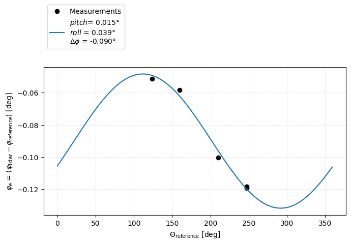
Now we see, that the external misalignment ($pitch, roll$) are <0.05°. A better alignment of the lidar could be perfromed by correcting the misalingment.

The static elevation offset ($\Delta \varphi$) has a value of -0.090°, which is considerable and might need to be considered for the stearing of the lidar. A negative $\Delta \varphi$ means, the lidar is looking to far up, so if we would command an elevation of 0° with a perfectly aligned lidar, we would actually measure at an elevation of 0.09°. This means a misalignment of 17.5m at 10km range.

Perform fit with Uncertainties and Monte Carlo Propagation

However, the actual measures of polar coordinates are prone to uncertainties.

Uncertainties in the measurement of the elevation and azimuth can be manifold:

• limited discretization of elevation and azimuth for lidar/theodolit

• Uncertainty in reading the “same” corner of the hard target scan from lidar

• pointing uncertainty of the thodolite (reference)

• … and others

The provided uncertainties just give an approximate indication and we do not claim them to be realistic.

💡 Info: This methodology has not been tested, verified nor published. If used, please cite this documentation.

Monte Carlo Uncertainty propagation

To propagate these uncertainties onto the fit results, we perform N_mc = 1000 monte carlo loops, where we sample random errors from a gaussian, defined by the provided uncertainties around their mean. A fit is performed for each of the loops, uncertainties in the resulting parameters $pitch,roll,\Delta \varphi$ are obtained as standard deviation from the distribution of the resulting parameters.

from lidalign.hard_target_elevation_mapping import HardTargetMappingElevation

HTM = HardTargetMappingElevation(df['Theo_Azimuth'].values, 
                           df['Delta Ele'].values, 
                           df['Unc_azi'].values, df['Unc_ele'].values
                           )


HTM.fit(typ = 'Other')
print(HTM.params)
fig, ax = plt.subplots(figsize = (4,3), dpi = 300)
ax = HTM.plot(ax= ax)
ax.set(title = None)

       mean   std    form
0  123.6162  0.02  normal
1  159.9877  0.02  normal
2  247.1387  0.02  normal
3  210.3619  0.03  normal
4  247.1331  0.03  normal
     mean   std    form
0 -0.0513  0.02  normal
1 -0.0582  0.02  normal
2 -0.1182  0.02  normal
3 -0.1004  0.03  normal
4 -0.1193  0.03  normal
Other

[ 0.01545298  0.03869653 -0.09008265]
(1000, 360)

[Text(0.5, 1.0, '')]

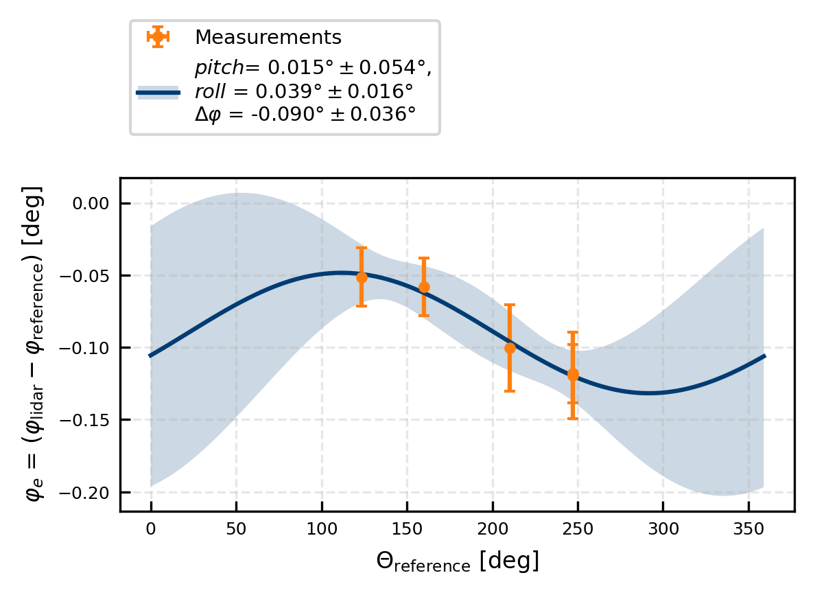
We can clearly see, that the elevation difference (between commanded and actual elevation) becomes up to -0.12° for certaint azimuths. The uncertainty of the elelvation difference becomes larger at azimuths, where we cannot verify the pointing accuracy due to missing hard targets for the fit. Thus, the uncertainty becomes smaller in the azimuth range with hard targets to observe.

An improvement can be obtained with more hard targets at varying azimuth angles .

🔔 Important: Note, that errors in the azimuth are considered, but are so small, that they do not appear.